Monday, 25 April 2016

FIR FILTER USING WINDOW FUNCTION

It is a filter whose impulse response if of finite duration. We have implemented this filter for linear phase using both C programming and Scilab.
     We used C programming to find impulse response h(n). Attenuation in passband and stopband (As,AP), passband and stopband frequencies(fS,fP) and sampling frequency(FS) were taken as inputs. From these values desired impulse response function was calculated and was then multiplied by the window function. The window function is decided from the value of As. The As of window function should be greater than that of the input.
     Scilab was used to plot the magnitude spectrum and phase spectrum of the FIR filter.
     As we take window function with higher As value, the side lobe width goes on decreasing with increasing main lobe width. The phase response of the filter is linearly varying with frequency and no distortion is observed in the output. The output is same as input delayed by some constant.
 
https://drive.google.com/drive/folders/0BwJUrR8ne7NkY21ycmFDRVpWSk0
FIR FILTER DESIGN USING FREQUENCY SAMPLING METHOD

 The objective of this experiment was to design a digital filter for the given input specifications using frequency sampling method. In this method the desired frequency response Hd(w) is sampled at w=2*pi*k/N ( where N = length of  the signal) The frequency samples are thus obtained are taken as DFT coefficients H[k]. FIR filter response is found by taken IDFT of H[k]. Magnitude and phase spectrum were plotted for this. Pass band and stop band attenuation values were verified.

https://drive.google.com/drive/folders/0BwJUrR8ne7NkRk44MTZCZWQwVGc


BASIC OPERATIONS USING DSP PROCESSOR

We studied programming on a DSP kit using Assembly Level Language. The kit used was TMS320F28375. This was demonstrated by a senior in our class. Instructions required for Arithmetic, Logical and Shift Operations were demonstrated. The changes in the values of the registers before and after execution of each operation were observed. The DSP was programmed using Code Composer Studio.


DIGITAL CHEBYSHEV FILTER DESIGN

Chebishev filters are analog or digital filters.they have ripples in passband or stop band depending upon their type.

There are two types of filters:
a) Type 1
b) Type 2 

Type 1:  
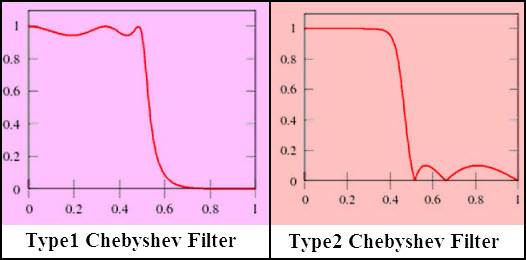
It has steeper roll-off in stop band, whereas passband has ripples
  
Type 2: 
Type 2 is exactly opposite to type1.Response is flat in passband and ripples cain in stop band.
   
 Figure above shows the response of type1 and type2 chebyshev filter .


Ripples for odd and even order of filter is shown .

We performed Type I low pass filter using Scilab. We first designed analog filter from the inputs and then designed digital filter from the analog filter. Attenuation in passband and stopband(AS,AP), passband and stopband frequencies(fS,fP) and sampling frequency(FS) were taken as inputs and we used to get magnitude spectrum and pole-zero plot for both analog and digital filter.
We observed that as we increase the order of filter, the ripples in passband reduce and we get more idealized characteristics. As all poles were inside the unit circle, the filter designed was stable.
https://drive.google.com/drive/folders/0BwJUrR8ne7NkNDhQU201cnlCZ0E

 ANALOG AND DIGITAL BUTTERWORTH FILTER DESIGN

Butterworth filter is designed to have passband and stopband as flat as possible. We implemented low pass Butterworth filter using Scilab. Attenuation in passband and stopband (AS,AP), passband and stopband frequencies(fS,fP) and sampling frequency(FS) were taken as inputs. First we designed analog filter from the inputs and then digital filter was designed from the analog filter. We got magnitude plot and pole-zero plot for both analog and digital filters in th output.


We observed that as we increase the order of the filter, magnitude plot becomes steeper in the transition band and we get more idealized plot. As all poles were inside the unit circle, the filters were stable.
As shown in the figure, for order N=11, we get response which tending to ideal one.
https://drive.google.com/drive/folders/0BwJUrR8ne7NkMkREVm9oSS1nZEU

 Overlap add and overlap save method

overlap add and overlap save method is the traditional name for an efficient way to evaluate the
discrete convolution between a very long signal x[n] and a finite impulse response  (FIR) filter h[n].
y[n] = x[n] * h[n] \ \stackrel{\mathrm{def}}{=} \ \sum_{m=-\infty}^{\infty} h[m] \cdot x[n-m] = \sum_{m=1}^{M} h[m] \cdot x[n-m],\,


where h[m]=0 for m outside the region [1, M].

We divided x(n) into small sequences of equal lengths and convoluted with h(n). Depending on which method is used, decomposed y(n) for both OAM and OSM were calculated.
 Though FFT yields  faster results it cannot be used in practice as it requires the entire length of the input signal which isn't possible as it would introduce large delay and memory requirements of the system will also increase. Hence, OAM and OSM are preferred.

https://drive.google.com/drive/folders/0BwJUrR8ne7NkUk1ReW9JV3RHQW8
FFT:

An algorithm for fast computation of DFT is FFT(Fast Fourier Transform).The algorithm which we have implemented can only calculate FFT for signal length of 4 of Radix-2. The FFT algorithm divides the N-point DFT input signal into 2 parts-even and odd signal values of the input. The even signal values can be directly found out whereas the odd signal values is just multiplied by an appropriate twiddle factor which overall reduces the complex multiplications for FFT. This happens because the signal is divided into 2 parts, so the computation is carried out only for N/2 signal values. This increases the speed of computations and makes FFT faster than other algorithms.

 
https://drive.google.com/drive/folders/0BwJUrR8ne7NkTlI5X2RvVTh6UEU